Overview

This page provides an overview of the models and methods implemented in regenie. A full description is given in our paper.

regenie carries out genome-wide association tests for both quantitative and binary (case-control) phenotypes. It is designed to handle

1. A large number of samples. For example, it is ideally suited to the UK Biobank dataset with 500,000 samples.
2. A combination of genetic data from a micro-array, imputation and exome sequencing.
3. A large number of either quantitative traits (QTs) or binary (case-control) traits (BTs)
4. Accounting for a set of covariates

An overview of the regenie method is provided in the figure below. Essentially, regenie is run in 2 steps:

1. In the first step a subset of genetic markers are used to fit a whole genome regression model that captures a good fraction of the phenotype variance attributable to genetic effects.
2. In the second step, a larger set of genetic markers (e.g. imputed markers) are tested for association with the phenotype conditional upon the prediction from the regression model in Step 1, using a leave one chromosome out (LOCO) scheme, that avoids proximal contamination.

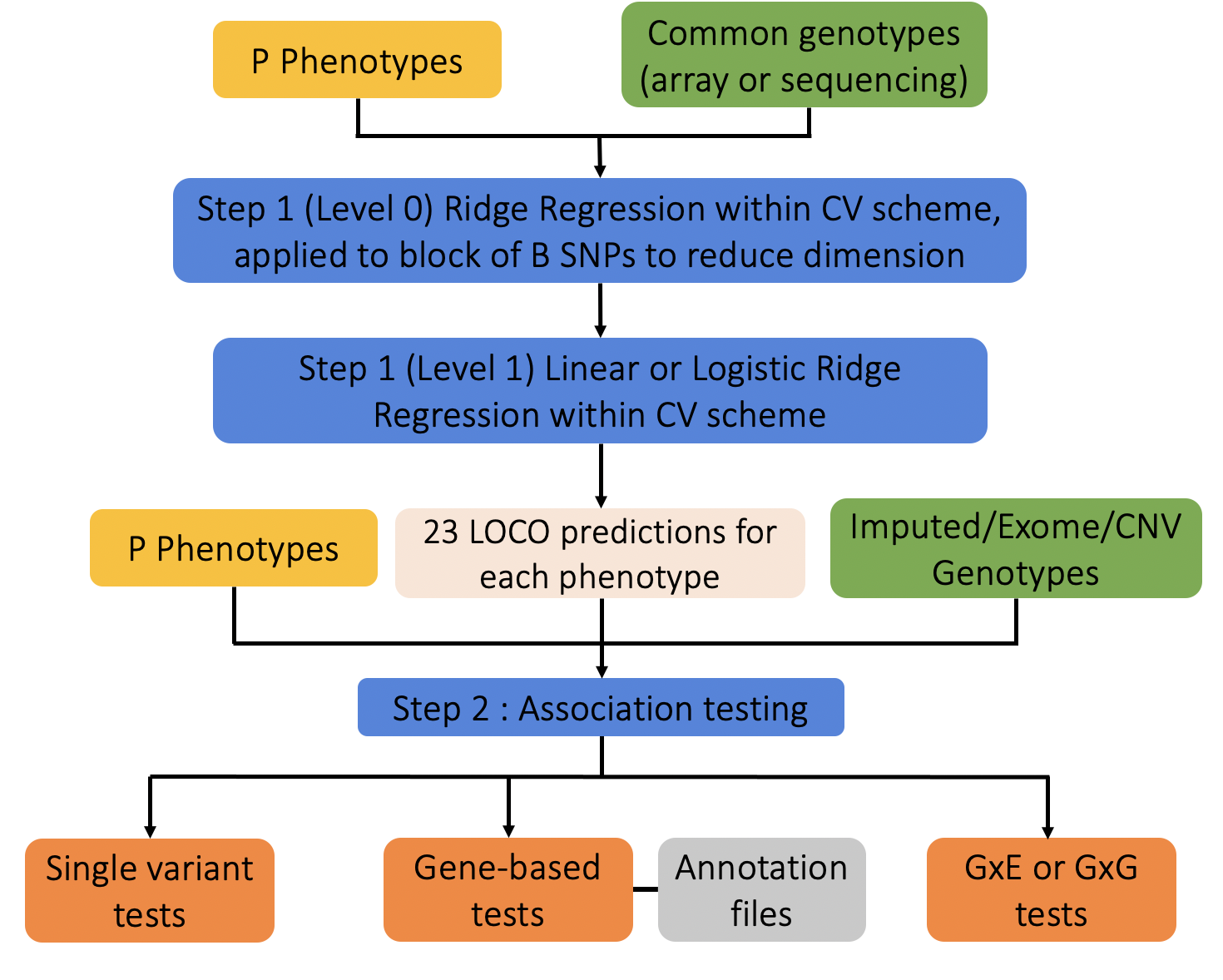
Step 1 : Whole genome model

In Step 1 a whole genome regression model is fit at a subset of the total set of available genetic markers. These are typically a set of several hundred thousand ($M$) common markers from a micro-array.

Ridge regression (level 0)

regenie reads in the $M$ markers in blocks of $B$ consecutive markers (--bsize option).

In each block, a set of ridge regression predictors are calculated for a small range of $J$ shrinkage parameters $\{\tau_1,\ldots, \tau_J\}$ (using --l0 option [default is 5]) .

For a block of SNPs in a $N\times B$ matrix $X$ and $N\times 1$ phenotype vector $Y$ we calculate $J$ predictors

$X\widehat{\beta}_1 \ldots, X\widehat{\beta}_J$

where

$\widehat{\beta}_j = (X^TX+\tau_j I)^{-1}X^T Y$

The idea behind using a range of shrinkage values is to capture the unknown number and size of truly associated genetic markers within each window. The ridge regression takes account of Linkage disequilibrium (LD) within each block.

These predictors are stored in place of the genetic markers in matrix $W$, providing a large reduction in data size. For example, if $M=500,000$ and $B=1,000$ and $J=5$ shrinkage parameters are used, then the reduced dataset will have $JM/B=2,500$ predictors.

Ridge regression is used in this step for both quantitative and binary traits.

Cross-validation (level 1)

The predictors generated by the ridge regression step will all be positively correlated with the phenotype. Thus, it is important to account for that correlation when building a whole genome wide regression model.

When analyzing a quantitative trait we use a second level of ridge regression on the full set of $JM/B$ predictors in $W$. This approach is inspired by the method of stacked regressions¹.

We fit the ridge regression for a range of shrinkage parameters (--l1 option) and choose a single best value using K-fold cross validation scheme. This assesses the predictive performance of the model using held out sets of data, and aims to control any over-fitting induced by using the first level of ridge regression to derive the predictors.

In other words, we fit the model

$$Y = W\alpha + \epsilon$$

where $\alpha$ is estimated as $\widehat{\alpha} = (W^TW + \phi\,I)^{-1}W^TY$ and the parameter $\phi$ is chosen via K-fold cross-validation.

For binary traits, we use a logistic ridge regression model to combine the predictors in $W$

$$\text{logit}(p) = \mu + W\alpha$$ where $p$ is the probability of being a case and $\mu$ captures the effects of non-genetic covariates.

Genetic predictors and LOCO

Once $\alpha$ has been estimated we can construct the genetic prediction

$$Z = W\widehat{\alpha}$$

Also, since each column of the matrix $W$ will be associated with a chromosome we can can also construct a genetic prediction ignoring any one chromosome, by simply ignoring those columns when calculating the prediction. This is known as the Leave One Chromosome Out (LOCO) approach. These LOCO predictions are valuable at Step 2 of regenie when each marker is tested for associated (see below).

For binary traits, it is the linear predictor in a logistic regression model using LOCO that is saved, and used as an offset when fitting logistic regression models to test for association.

Multiple phenotypes

The dimension reduction step using ridge regression can be used very efficiently to model multiple phenotypes at once. The ridge regression equations for a block of SNPs in a $N\times B$ matrix $X$ and a single phenotype in a $N\times 1$ matrix $Y$ take the form

$\widehat{\beta} = AY$ where $A = (X^TX+\tau I)^{-1}X^T$ does not depend on $Y$

If instead $P$ phenotypes are stored in columns of a $N\times P$ matrix $Y$, then the matrix $A$ can be applied jointly to calculate the matrix of estimates $\widehat{\beta} = AY$, and this can take advantage of parallel linear algebra implementations in the Eigen matrix library.

Covariates

Covariates, such as age and sex and batch effect variables can be included in the regenie model.

For quantitative traits, any covariates are regressed out of phenotypes and genotypes before fitting the model.

For binary traits, we fit a null model with only covariates, and use predictions from that model as an offset when fitting the logistic regression model.

Step 2 : Single-variant association testing

In Step 2, a larger set of markers are tested for association with the trait (or traits). As with Step 1, these markers are also read in blocks of $B$ markers, and tested for association. This avoids having to have all markers stored in memory at once.

Quantitative traits

For quantitative traits, we use a linear regression model for association testing.

• Covariates are regressed out of the phenotypes and genetic markers.
• The LOCO predictions from Step 1 are removed from the phenotypes.
• Linear regression is then used to test association of the residualized phenotype and the genetic marker.
• Parallel linear algebra operations in the Eigen library are used where possible.

Binary traits

For binary traits, logistic regression score test is used to test association of the phenotype and the genetic marker.

The logistic regression model includes the LOCO predictions from Step 1 as an offset. Covariates are included in the linear predictor in the usual way.

When the case-control ratio is imbalanced, standard association tests don't control Type I error well at rare genetic markers. regenie has two options to handle this

Firth logistic regression

Standard maximum likelihood estimates are generally biased. The Firth correction² removes much of the bias, and results in better calibrated test statistics. The correction involves adding a penalty term to the log-likelihood,

$$\widetilde{l}(\theta) = l(\theta) + {1 \over 2} \log I|\theta|$$

where the penalty term corresponds to the use of Jeffrey's Prior. This prior has the effect of shrinking the effect size towards zero.

regenie uses a Firth correction when the p-value from the standard logistic regression test is below a threshold (default 0.05). It also includes a novel, accurate and fast approximate Firth correction which is ~60x faster than the exact Firth correction (see the option --firth).

The p-value reported in regenie is based on a likelihood ratio test (LRT), and we use the Hessian of the log-likelihood without the penalty term to estimate the standard error (SE). This may cause an issue in meta-analyses with rare variants, as the effect size estimate and SE may not match with the LRT p-value. Hence, we added an option --firth-se to report a SE computed instead from the effect size estimate and the LRT p-value.

Saddle point approxiation (SPA) test

The SPA test approximates the null distribution of the test statistic by approximating the cumulant generating function of the test statistic, which involves all of the higher order moments³$^,$⁴. This provides a better estimation of the tail probabilities compared to using standard asymptotic theory which relies on the normal approximation and uses only the first two moments of the dsitribution. A tail probability is obtained as

$$\begin{align*} P&(T < t_{\text{obs}}) \approx \Phi(z), \text{ where,}\\ z &= w + \frac{1}{w}\log{\frac{v}{w}}\\ w &= \text{sign}(\delta^*)\sqrt{ 2 [ t_{\text{obs}}\, \delta^* - K(\delta^*)}],\, v = \delta^*\sqrt{K''(\delta^*)} \end{align*}$$

and $K(\delta)$ is the cumulant generating function of the test statistic and $\delta^*$ is obtained by using a root-finding algorithm for $K'(\delta)=t_{\text{obs}}$. As this approximation has been found not to work very well for ultra-rare variants, a minimum minor allele count (MAC) is used to filter out these variants before testing (option --minMAC).

Step 2 : Gene-based testing

Instead of performing single-variant association tests, multiple variants can be aggregated in a given region, such as a gene, using the following model

$$g(\mu) = w_1G_1\beta_1 + \dots + w_mG_m\beta_m$$

where $G_i$'s represent the single variants included in the test, $w_i$'s and $\beta_i$'s are weights and effect sizes, respectively, for each variant, and $g(.)$ is a link function for the phenotypic mean $\mu$. We also denote by $S_i$ the score statistics obtained from the single-variant tests. This can be especially helpful when testing rare variants as single-variant tests usually have lower power performance.

To avoid inflation in the gene-based tests due to rare variants as well as reduce computation time, we have implemented the collapsing approach proposed in SAIGE-GENE+⁵, where ultra-rare variants are aggregated into a mask. For highly imbalanced binary traits, SPA/Firth correction can be used to calibrate the test statistics in the gene-based tests as proposed in Zhao et al. (2020)⁶ using --firth/--spa.

Burden tests

Burden tests, as defined in Lee et al. (2014)⁷, assume $\beta_i=\beta\; \forall i$, where $\beta$ is a fixed coefficient, which then leads to the test statistic $$Q_{BURDEN} = \left(\sum_i w_iS_i\right)^2$$ These tests collapse variants into a single variable which is then tested for association with the phenotype. Hence, they are more powerful when variants have effects in the same direction and of similar magnitude. In regenie, multiple options are available to aggregate variants together into a burden mask beyond the linear combination above (see here). For example, the burden tests that were employed in Backman et al. (2021)⁸ use the default strategy in regenie of collapsing variants by taking the maximum number of rare alleles across the sites.

Variance component tests

Unlike burden tests, SKAT⁹ assume the effect sizes $\beta_i$ come from an arbitrary distribution with mean 0 and variance $\tau^2$ which leads to the test statistic $$Q_{SKAT} = \sum_i w_i^2S_i^2$$ Hence, SKAT can remain powerful when variant effects are in opposite directions.

The omnibus test SKATO¹⁰ combines the SKAT and burden tests as $$Q_{SKATO} = \rho Q_{BURDEN} + (1-\rho) Q_{SKAT}$$ So setting $\rho=0$ corresponds to SKAT and $\rho=1$ to the burden test. In practice, the parameter $\rho$ is chosen to maximize the power [regenie uses a default grid of 8 values {$0, 0.1^2, 0.2^2, 0.3^2, 0.4^2, 0.5^2, 0.5, 1$} and set the weights $w_i = Beta(MAF_i,1,25)$].

To obtain the p-value from a linear combination of chi-squared variables, regenie uses Davies' exact method¹¹ by default. Following Wu et al (2016)¹², regenie uses Kuonen's saddlepoint approximation method¹³ when the Davies' p-value is below 1e-5 and if that fails, it uses Davies' method with more stringent convergence parameters (lim=1e5,acc=1e-9).

The original SKATO method uses numerical integration when maximizing power across the various SKATO models that use different values for $\rho$. We also implement a modification of SKATO, named SKATO-ACAT, which instead uses the Cauchy combination method¹⁴ to combine the p-values from the different SKATO models.

Cauchy combination tests

The ACATV¹⁵ test uses the Cauchy combination method ACAT to combine single variant p-values $p_i$ as $$Q_{ACATV} = \sum_i \widetilde{w}_i^2\tan{\{\pi(0.5 - p_i)\}}$$ where we set $\widetilde{w}_i = w_i \sqrt{MAF(1-MAF)}$. This test is highly computationally tractable and is robust to correlation between the single variant tests.

The omnibus test ACATO¹⁵ combines ACATV with the SKAT and burden tests as $$Q_{ACATO} = \frac{1}{3}\tan{\{\pi(0.5 - p_{ACATV})\}}+ \frac{1}{3}\tan{\{\pi(0.5 - p_{Burden})\}}+ \frac{1}{3}\tan{\{\pi(0.5 - p_{SKAT})\}}$$

where unlike the original ACATO test, we only use one set of the weights $w_i$. Alternatively, we augment the test to include an extended set of SKATO models beyond SKAT and Burden (which correspond to $\rho$ of 0 and 1 in SKATO respectively) and use the default SKATO grid of 8 values for $\rho$.

Sparse Burden Association Test

regenie can generate burden masks which are obtained by aggregating single variants using various annotation classes as well as allele frequency thresholds. The Sparse Burden Association Test (SBAT)¹⁶ combines these burden masks in a joint model imposing constraints of same direction of effects $$\mu = \sum_{\text{mask }i} M_i\gamma_i$$ where $M_i$ represent a burden mask and we solve $$\underset{\boldsymbol\gamma}{\min} || Y - \sum_i M_i\gamma_i||^2 \text{ subject to } \gamma_i \ge 0 \text{ for all } i$$

The SBAT method tests the hypothesis $H_0: \gamma_i=0$ for all $i$ vs. $H_1: \gamma_i > 0$ for some $i$. By using this joint model, the SBAT test accounts for the correlation structure between the burden masks and with the non-negative constraints, it can lead to boost in power performance when multiple burden masks are causal and have concordant effects. This test has the nice property that it combines model selection of the masks (via the sparsity induced by the non-negative assumption) with model inference (it is well calibrated and powerful).

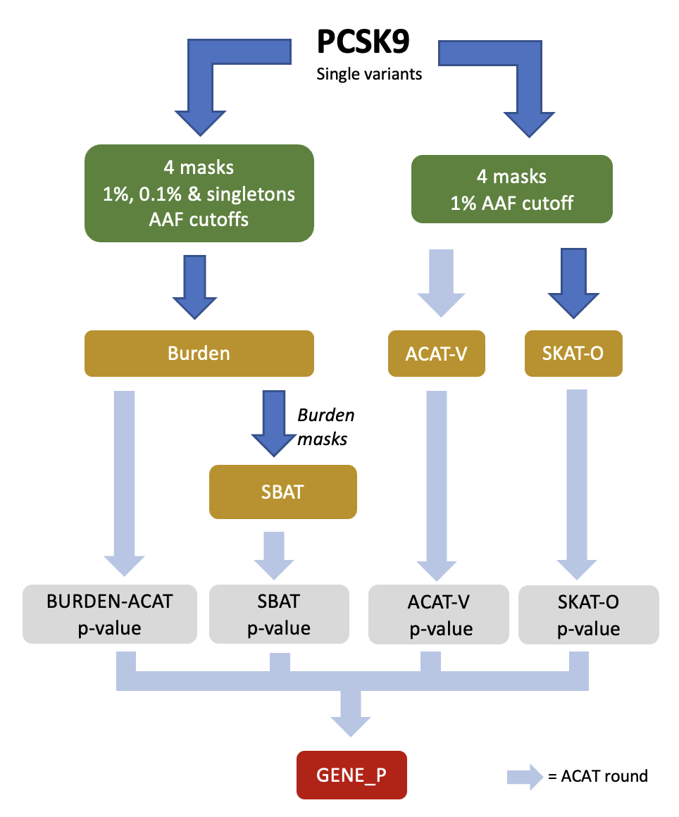
GENE_P

As the different gene-based tests in REGENIE can be more powerful under different genetic architectures, we propose a unified strategy, named GENE_P, that combines the strengths of these tests. It uses ACAT to combine the p-values of the SKATO, ACATV, Burden and SBAT tests and obtain an overall assessment of significance for a genetic region (e.g. gene). The diagram below illustrates the GENE_P test using 4 masks (i.e. combination of variant annotations) and 3 allele frequency cutoffs when performing gene-based tests.

Step 2 : Interaction testing

The GxE tests are of the form $$g(\mu) = E\alpha + G\beta + (G\odot E)\gamma$$ where $E$ is an environmental risk factor and $G$ is a marker of interest, and $\odot$ represents the Haddamard (entry-wise) product of the two. The last term in the model allows for the variant to have different effects across values of the risk factor. Note: if $E$ is categorical, we use a dummy variable for each level of $E$ in the model above.

We can look at the following hypotheses:

1. $H_0: \beta = 0$ given $\gamma = 0$, which is a marginal test for the SNP
2. $H_0: \beta = 0$, which is a test for the main effect of the SNP in the full model
3. $H_0: \gamma = 0$, which is a test for interaction
4. $H_0: \beta = \gamma = 0$, which tests both main and interaction effects for the SNP

Misspecification of the model above, such as in the presence of heteroskedasticity, or the presence of high case-control imbalance can lead to inflation in the tests. Robust (sandwich) standard error (SE) estimators¹⁷ can be used to adress model misspecification however, they can suffer from inflation when testing rare variants or in the presence of high case-control imbalance¹⁸$^,$¹⁹.

In regenie, we use a hybrid approach which combines:

• Wald test with sandwich estimators
• Wald test with heteroskedastic linear models (for quantitative traits)
• LRT with penalized Firth regression (for binary traits)

For quantitative traits, we use the sandwich estimators HC3 to perform a Wald test for variants whose minor allele count (MAC) is above 1000 (see --rare-mac). For the remaining variants, we fit a heteroskedastic linear model (HLM)²⁰ $$Y = E\alpha + E^2\zeta + G\beta + (G\odot E)\gamma + \epsilon$$

where we assume $\epsilon \sim N(0, D)$ where $D$ is a diagonal matrix with entries $\sigma^2\exp{(1 + E\theta_1 + E^2\theta_2)}$. This formulation allows for the phenotypic variance to also depend on the risk factor $E$. By incorporating both the linear and quadratic effect of $E$ in the mean and variance of $Y$, this model provides robustness to heteroskedasticity (Note: the $E^2$ terms are only added when $E$ is quantitative). Wald tests are then performed for the null hypotheses listed above.

For binary traits, we consider the following interaction model $$\text{logit}(\mu) = E\alpha + E^2\zeta + G\beta + (G\odot E)\gamma$$ where we also include a non-linear effect for $E$ (not if categorical). The sandwich estimator HC3 is used in a Wald test for variants whose MAC is above 1000 (see --rare-mac) otherwise the model-based standard errors are used. When Firth is specified, we only apply the Firth correction using LRT if the p-value for the interaction term $\gamma$ from the Wald test is below a specified threshold (see --pThresh). So the added $E^2$ term as well as the use of the Firth penalty help with case-control imbalance and model misspecification for the effect of $E$ on the phenotype.

Missing Phenotype data

With QTs, missing values are mean-imputed in Step 1 and they are dropped when testing each phenotype in Step 2 (unless using --force-impute).

With BTs, missing values are mean-imputed in Step 1 when fitting the level 0 linear ridge regression and they are dropped when fitting the level 1 logistic ridge regression for each trait. In Step 2, missing values are dropped when testing each trait.

To remove all samples that have missing values at any of the $P$ phenotypes from the analysis, use option --strict in step 1 and 2. This can also be used when analyzing a single trait to only keep individuals with complete data by setting the phenotype values of individuals to remove to NA.

Note: imputation is only applied to phenotypes; covariates are not allowed to have missing data.

References